The purpose of this review is to provide a rough outline of the topics that
were most necessary for the
homeworks and to recall other important notions. This review is "unofficial"
(meaning, the instructor had
no input), but will hopefully be a good list of core concepts one should strive
to understand prior to the first
midterm. Please cross reference the instructor's notes as well as the book for
other key topics, examples,
and definitions!
1 Linear Equations
1.1 Linear Equations and Their Solution
We begin by motivating the subject of linear algebra by asking the question,
"what x, y, and z can I plug
into the equations,
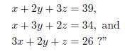
The question is interesting, but not exhaustive. Instead, we look to ask if
there are any solutions to this
system of equations , and IF so, how many?
(a) First we note that there are two types of systems that can occur. Namely,
homogeneous systems and
inhomogeneous systems. How do these differ? Morevoer, we learn other important
definitions such
as consistent, inconsistent, solution set, general solution, trivial solution.
leading term, free variables,
linear equation, and equivalent equations .
(b) However, the difficult nature of simply adding and substracting entire
equations is cumbersome and is
one motivation for learning to utilize matrices. This leads to the next section.
1.2 Matrices and Echelon Forms
(a) When creating matrices to solve systems of equations (as in the situation
above), we place the `unkowns'
on the left side of the matrix and the 'equals' part on the right side of some
sort of divider. This matrix
is then called an augmented matrix.
(b) Howver, we will also use matrices without such dividers, these are simply
called coefficient matrices.
Note that in both cases, we exclude the variables from the matrices . We use only
the coefficients.
(c) Next, we aim to simplify the matrix. To do this, we are allowed to
perform the following elementary
row operations: scaling ( multiplying an equations by a nonzero scalar),
exchanging two equations, and
elimination (add a multiple of one equation to another).
(d) (Various echelon forms:) Now we explore the terminology behind different
types of `simplified' matrices.
Rather than list definitions, let us view an example: for the matrix
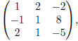
we have
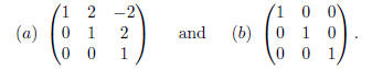
Here, (a) is the echelon form of the matrix, and (b) is the matrix in reduced
echelon form.
(e) When reducing matrices into echelon and reduced echelon forms in order to
solve systems of equations,
we find that three things can happen (here I use terminology assuming that after
reducing the matrices
into echelon form we then switch back to dealing with the variables):
(i) (Unique Solution:) If, after reducing, we have found that each
variable is equal to a number (or
letter, etc.), we say that it is a unique solution.
(ii) (Infinitely Many Solutions:) If, after reducing, we are left with any of
our variables in terms of
other variables (at least one free variable), we say this system has infinitely
many solutions.
(iii) (No Solutions:) If, after reducing, we are left with an inconsistency,
i.e., something of the form
0=3, we say the system has no solutions.
(f) Note then, that if we have an augmented matric for a homogenous sytem of
equations, that is, every
element in the column right of the divider is a 0, then it is impossible
to get an inconsistency. In other
words, a homogenoues system of equations always has at least one
solution, namely the trivial solution.
(g) Be sure to feel comfortable with what the theorems in this chapter are
saying. These theorems are
explaining under what conditions we have either infinitely many solutions, a
unique solution, or no
solutions.
2 The Vector Space Rn
2.1 Vectors and the Space Rn
(a) Here we learn what a vector is, when two vectors equal
one another, how to add and subtract vectors ,
and how to multiply vectors by scalars. Moreover, we are introduced to the zero
vector , which is
simply a vector with every entry being a zero. Note that if two vector are of
different sizes , then the
operations of adding and subtracting are not defined.
(b) The standard basis of Rn is introduced in
this chapter as well. We will learn a lot more about bases
as the quarter continues. However, throughout the quarter we will consistently
use the standard basis
becuase it is very easy to manipulate (add, multply, etc.) these vectors.
(c) Know the definition of linear combination!!!!!
Understand how answering the question "can this vector
be written as a linear combination of those vectors" be translated into matrix
form and solved in this
manner!!!
2.2 The Span of a Sequence of Vectors
(a) Note that given a set of vectors
 we can take a linear combination of these
vectors,
we can take a linear combination of these
vectors, 
 and possibly create a new vector u that is
not any of the vectors in our set. Changing
and possibly create a new vector u that is
not any of the vectors in our set. Changing
the scalars  in the linear combination above
would result in yet another vector! We call
in the linear combination above
would result in yet another vector! We call
the collection of all linear combinations of our set of vectors the span
of  and denote this
collection Span  Understanding this is very
important.
Understanding this is very
important.
(b) Therefore, we find that asking whether or not a vector
is in the span of a set of other vectors is the
same as asking whether that vector can be written as a linear combination of the
other vectors. The
way in which we can solve this using matrices is then the same as last section.
(c) Another question one may want to ask is given a set of
vectors in Rn, does this set of vectors span
Rn? That is, can every vector in Rn be written as a linear
combination of the vectors in this set? To
answer this question we have the following theorem:
(d) (A Criterion for Spanning Rn) Let A be an
n*k matrix with columns  Then the
following are equivalent:
(i) Span 
(ii) For every n-vector b the system o flinear equations with augmented matrix
[A | b] is consistent.
(iii) Every n-vector b is a linear combination of

(iv) A has n pivots positions (equivalently, every row contains a pivot).
Note, in terms of answering the question above, we usually
show (iv) holds, thus implying (i).
(e) We also learn the definition of a subspace and also
knowledge of certain conditions in which the span
of two different sets of vectors may be equal (Lemma 2:27 in my book).
2.3 Linear Independence in Rn
(a) Know the definition of linear independece and linear
dependence very very well!
(b) We learn that if
are n-vectors, then they are linearly independent if, and only if, the matrix
 with columns
has k pivots, one for each column.
with columns
has k pivots, one for each column.
(c) Moreover, if we have n vectors
 then the matrix A above is a square matrix
and we
then the matrix A above is a square matrix
and we
have the vectors are linearly independent if, and only if, there are n pivots.
But ALSO we have that
these vectors span Rn if, and only if, they are linearly independent!
(d) If a set of vectors are linearly dependent, then we
can throw out vectors until we are left with a set of
linearly independent vectors. On the other hand, if we have a set of linearly
independent vectors and
we also have another vector that is not a linear combination of these
vector, then the set of vectors
along with this new vector is again linearly independent.
2.4 Subspaces and Bases of Rn
(a) Here we learn the definitions of closed under
addition, closed under multiplication subspace, basis,
dimension, and coordinate vector . What is the difference between a basis of Rn
and a basis of a
susbspace?
(b) The definitions of most of these words is defined with
respect to the spaces of Rn. In the future, we will
generalize these definitions slightly for spaces that aren't necessarily Rn. As
an example of something
that is not closed under addition in a space other that Rn, consisder
the `space' of 'likes'. Take two
things from your 'likes' space, i.e., 'significant other' and 'best friend'.
Individually you may like both
of them, but if they ever got together, you may dislike that!
(c) Be able to show whether or not a given subset of Rn
is a subspace or not.
(d) A basis of Rn is a set of vectors in Rn
such that these vectors are linearly independent and this set
of vectors span Rn. Note that a basis amounts to being the smallest
amount of vectors that still span
Rn. However, also note that a basis is not unique. In other words, a
space can have many many bases!
(e) If we write an arbitrary vector u in Rn as
a linear combination of some basis vectors  in a
in a
basis β, that is,  then placing the
coefficients
then placing the
coefficients  into a vector produces
the coordinate vector of u with respect to β. Note that a different basis, β,
would produce a different
coordinate vector.
2.5 Geometry of Rn
(a) Be comfortable calculating dot products,
norm/length/magnitude, distance, the angle between two vectors, the projection
of one vector onto another, the orthogonal complement, and the projection of one
vector orthogonal to another.
(b) Each of the above has a formula involved with it along
with a geometrical interpretation. For example,
how can one find if two vector are orthogonal? How can we find if a vector is a
unit vector? If
normalizing a vector is dividing each component of a vector by its length, what
does this do to the
vector geometrically?
c) Recall thetriangle inequality which states for any two
vector u, v in Rn, 
Meanwhile, the Cauchy-Schwartz inequality gives that for for any two vectors u,
v in Rn, we have

3 The Algebra of Matrices
3.1 Introduction to Linear Transformations and Matrix
Multiplication
(a) In this section we learn what the definitions are for
functions, maps, domain, range, linear transformations, standard matrix, and
matrix tansformation.
(b) If asked to show somehting is a linear tranformation,
what would you do?
(c) In short, we find that if we have a function T :
 that satisfies the properties such that for
all
that satisfies the properties such that for
all
u and v in Rn and  we have T(u +
v) = T(u) + T(v) and T(cu) = cT (u), we call this function
we have T(u +
v) = T(u) + T(v) and T(cu) = cT (u), we call this function
a linear tranformation. It ends up that matrices can also satisfy these
conditions. Along with the fact
that matrices map vectors from  where n and m
are determined by the size of the matrix,
where n and m
are determined by the size of the matrix,
we have that some matrices can be viewed as linear transformations!
(d) The definition of a linear transformation is basically
saying that is is a particular function such that it
does not matter if we add the vectors in the range first then map, or map the
vectors and then add.
Similarly, it does not matter if we scalar multiply then map, or map and then
scalar multiply. Having
these properties if very useful.
3.2 The Product of a Matrix and a Vector
(a) We learn to multiply a matrix and vector together.
This is essiental to the course.
(b) The identity matrix for Rn is the n*n matrix with 1's on the
diagonal and 0's in every other entry.
(c) The null spubspace of an m*n matrix A consists of all n-vectors x such that
Ax = 0 and denoted
null (A). Also know what an affine subspace of Rn is!!
3.3 Matrix Addition and Multiplication
(a) Here we learn that adding matrices is as simple as
adding the components within matrices. Unfor-
tunately, multiplying two matrices requires much more work, but it'snot that
bad...(Just recall the
memory device -1, i.e., row with column).
(b) Many matrices will have nice properties in the future
based on where they have their entries. We
therefore have names such as zero matrix, square matrix, diagonal matrix, and
upper and lower diagonal
matrices as names for these matrices.
(c) Similarly, matrices that abide by certain properties
have names such as the negative , symmetric, and
skew symmetric. One should also know what the transpose of a matrix is and how
to compute it!
(d) CAUTION: Note that for two n*n matrices A and B we
always have A+B = B +A, we DO NOT
always have AB = BA!!!