A Math Primer

D. Bivariate Linear Regression

Introduction
One must be very careful however in how the
previous statistical approach is used. It is evident
from the data that the two variables studied
(atmospheric CO₂ and human population) are indeed
strongly correlated and that the variation in one
explains that of the other. But does this mean a true
functional dependency? Functional dependency
assumes that the magnitude of the dependent
variable (Y) is determined in part by the magnitude
of the independent variable (X). For example, in
studying the relationship between blood pressure
and age, it is reasonable to assume a functional
dependency, i.e. a person’s blood pressure depends
on their age (most of the time). This is not to
suggest age is the only factor responsible for
increases in blood pressure, and is not to suggest a
causal relationship is proven, but that age is one
possible determinant of blood pressure. One must
be particularly careful in interpreting
relationships (even strong ones).

In the example above, the observed relationship
between atmospheric CO₂ and human population
may be used to suggest that there exists a functional
dependency between these two variables through,
for example, increased respiration of human
populations (and thus larger releases of CO₂ to the
atmosphere). This, of course appears immediately as
a ludicrous statement that seems impossible to
sustain with a straight face. Indeed, although there
seems to be a functional dependency between these
two variables it is an indirect one, whereby human
population increase has lead large-scale
environmental changes such as fossil fuel
combustion and deforestation that themselves have
lead to increases fluxes of CO₂ (and other gases) to
the atmosphere.

More dangerous yet is the potential for spurious
correlations, the type of strong relationship between
two variables that can be completely explained by
independent arguments rather than a true functional
dependency (we call these arguments nested
relationships). One example of such spurious
correlation is presented below. Consider the growth
of two populations in the state of Georgia: humans
and storks. One can see from Figure 5 that there
exists a strong relationship between these two
variables and by running the previous exercise one
obtains a value of 0.99 for the coefficient of
determination (r²).

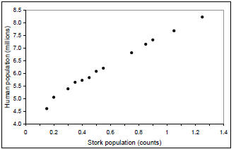
Fig. 4. Human vs. wood stork (Mycteria americana)
populations from 1970 to 2000 in the state of
Georgia.

This suggests that the variation in stork population
in the last 30 years in Georgia can explain most of
the variation in human population. In other words,
this relationship can help demonstrate that the
increase in the human population has been made
possible thanks to the increase of the stork
population in that state (which, if you believe Walt
Disney’s “Dumbo”, points to the primordial role of
these graceful birds in bringing human babies to
their final destination…) If there is isn’t a shred of
evidence in this past argument, one must also accept
that the observed relationship is somewhat
suspicious. By all means, one might expect a very
opposite effect of increased human population (and
thus land use expansion and habitat degradation,
added to increases in contaminant releases) on stork
populations. Indeed, Stork numbers presented here
represent sightings along a predetermined transect,
which is not equivalent to a full census of the stork
population in Georgia. This might just represent an
increased effort from the surveyors. Although a true
increase in the population cannot be excluded
(maybe through conservation efforts and
reinstallation of individuals in the population). In
any extent, a “perfect” relationship does not by any
means sustain causality in the variables studied.

Linear Regression Analysis
As with correlation, regression is used to analyze
the relationship between two continuous (scale)
variables. However, regression is better suited to
study the functional dependency between factors.
Also, the “products” (output) of regression and
correlation analyses differ. Put it very simply , with
regression, you are predicting the average change in
the dependent variable Y per unit independent
variable X, whereas with correlation you are
describing the fit of the two-dimensional scatter
(spread) around a trend line. To illustrate regression,
let’s use the same illustrative example as in the
previous section (global human population vs.
atmospheric CO₂).

Regression Model
The simplest functional relationship between two
variables is that of a linear relationship. Yu might
remember from algebra (see section above) that a
line is described by its intercept and slope:

y = ax + b

where y is the dependent variable, x is the
independent variable, a is the slope of the line (also
called m), and b is the intercept (where the line
crosses the Y-axis).

If all data were to fall on a straight line, drawing a
line that connects the data would be a trivial matter.
However, because we are dealing with statistical
scatter, choosing a line is not an easy matter. To
determine the best fitting line for the data set, let’s
assume:

represents the predicted value of Y
a represents the slope of the line
b represents the intercept of the line
The regression equation is :

= ax + b

Because of random scatter, each data point will be a
certain distance from the line. These distances, are
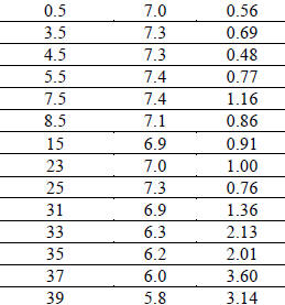
called error terms or residuals. To illustrate the
principles of regression, let’s use a data set of
chemical parameters in lake sediments: aluminum
and lignin content along the depth of a sediment
profile (0-40 cm). (Lignin is a natural organic
component exclusive to vascular plants and which is
used as a tracer for terrigenous inputs to aquatic
systems).

Sediment depth (cm)	Al (%)	Lignin (mg/g)

The residuals for this illustrative data set
represented by the vertical lines in Figure 5 below:

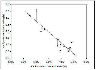
Fig. 5. Lignin concentrations (natural organic matter
exclusive to vascular plants) vs. aluminum
concentrations in lake sediments.

The strategy for determining the line is to select the
intercept (b) and slope (a) that minimizes the sum of
squared residuals . This is called the least squares
line. The slope of the least squares line is given by
the equation:

Where is the sum of the cross- products and
is the sum of squares for the variable X.
(remember that formulas for these sums of squares
were presented in the previous section).

For the illustrative data, = -6.26 and =
3.89 (you should test this by calculating these two
parameters). Therefore the slope a is:

The intercept of the line is:

where is the average value of the variables Y,
is the average value of the variables X, and a is the
slope of the line. Hence for the illustrative data set,



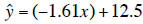
The regression model for the illustrative data set is
therefore:



Interpretation
In the previous section, we’ve learned how to
calculate the correlation coefficient (r) and the
coefficient of determination (r²). The correlation
coefficient for this data set is –0.91, which states
that there exists a rather strong negative relationship
between the two variables (in other words, any
increase in the independent variable, X, yields lower
values of the dependent variable, Y). The coefficient
of determination is 0.82 and states that 82% of the
variability of Y is explained by the variability of X.
To assess if this is indeed a relationship built on
functional dependency one must know something
about the system of study (and here geochemical
principles).

In short, aluminum is an abundant element in the
earth’s crust and is a predominant component of
small sized minerals operationally defined as clays
and mineralogically called aluminosilicates.
Generally, the percentage (or relative amount) of
aluminum increases inversely with respect to the
size of solid particles (i.e. sand fractions, >2mm,
will have very low amount of aluminum, whereas
clays, <2μm, will tend to have higher relative
proportions of aluminum ). Lignin, an organic
biomolecule exclusive to land plants, tends to occur
in high concentrations in woody tissues and in lower
amounts in soft tissues (i.e. leaves) and small plant
fragments. In a soil, for example, very small
particles (i.e. clays) will absorb small quantities of
organic matter including small amounts of lignin
components (from plant fragments). In contrast,
large plant macro-debris will be more enriched in
lignin components (but associated with sands that
are depleted in aluminum). In any extent, the
relationship observed in the studied lake sediments
suggest that the bottom of the lake receives a
changing proportion of large sandy particles
enriched in lignin (but depleted in aluminum) and
small clayey material enriched in aluminum (but
depleted in woody fragments). This relationship is
indeed functional and points to changes in the lake’s
drainage basin that lead to variations in material
inputs to its bottom (i.e. due to variations in storm
activities or other natural or human-based process).
Hence, it becomes clear that to demonstrate the
validity of an observed correlation, one must be able
to establish some sort of functional dependency
between the variables (whether direct or indirect),
and thus know something about the system of study.

An important aspect of regression analysis, aside
from establishing a relationship, is the calculation of
the slope of the model. The slope has a direct
interpretation as the predicted change in variable Y
per unit change in the variable X. In the case of a
linear correlation, the rate of change is constant
throughout the range of the data set. For the
illustrative example above, the slope of –1.61
suggests that for every additional unit in X
(percentage of aluminum in sediments), we predict a
decrease in Y (amount of lignin in sediments) of
1.61 units. The model can also be used to predict
values for Y given a known value of X. For
examples, if we were to analyze another sediment
sample and obtained an aluminum concentration of
5.5%, the predicted lignin content would be ~3.6
mg/g. Or, we could extrapolate the relationship to y
= 0 and solve to calculate the predicted amount of
aluminum in minerals with no lignin whatsoever.
The solution of this equation is 7.71% (you should
try to solve it).

This study is by far minimal in its analysis but
should act as a primer in starting work with linear
relationships between two variables. A more in
depth approach will help develop the concepts
necessary for quantitative analyses of problem sets.