Methods For Interval Linear Equations

5. Preconditioning

We now consider methods of preconditioning which allow a preconditioned equation to be
solved exactly in part or in whole. One type of method involves preconditioning a vector so
that it is SD. See the methods in Sections 6 and 7. Another type eliminates the variables
which are not SD so that the problem can be partially solved. The latter type can be
regarded as preconditioning so that certain quantities are zeroed. It involves operations by
an interval matrix, so it is perhaps misleading to call it preconditioning. See the methods
in Sections 8 and 9.

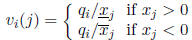
We now consider the first type of preconditioning. Assume an interval vector
is not SD. Define a real vector q with components



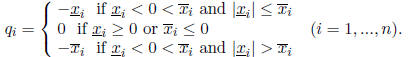
Then the interval vector y = x + q is the nearest SD interval vector to x in some sense.

Assume x is not SD. However, assume that at least one component of x is strictly SD. By
"strictly SD", we mean that the the interval is SD and neither endpoint is zero. An interval
having an endpoint which is zero is SD , but not strictly SD. Let j be the index such that
is the component of largest mignitude. The mignitude of is



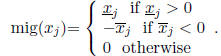
Define the vector v(j) with components



and define the matrix



Then is SD.
Note that

Therefore, is known exactly when has been determined.

In what follows, we do not actually use the interval vector (such as x) which we pre-
condition so as to be SD. Instead, we use an unspecified real vector . However, if we
precondition so that the interval vector x is SD, then the sign of any component of
has the sign we impose on the corresponding component of x.

Suppose we precondition a matrix A by multiplying by a real matrix . The product
can be irregular even when A is regular and is nonsingular. The four methods
we describe below all use some kind of preconditioning and in two cases becomes an
interval matrix. In each method, we assume that is such that M is regular.

A virtue of the preconditioning method just described is that the preconditioning matrix
differs from the identity in only one row. Contrast this with preconditioning using the inverse
of the center of A: See Section 1.

The matrix in (5.2) will be used as a preconditioner. The smaller the norm of the
vector v(j) used to define , the closer is to the identity. The enlargement of the
solution set by preconditioning is less when is nearer the identity.. If more than one
component of x is strictly SD, it is sometimes possible to define a matrix similar to
which is nearer the identity. We omit the details.

6. Third method

Our third method is obtained by introducing preconditioning into our first method. Suppose
we have obtained crude bounds x^B on the solution to Ax = b and find that at least one
component of x^B is SD. Then the corresponding component of the hull h is SD. Therefore
we can determine a matrix V as in Section 5 such that V x^B is SD. This assures that V h is
SD.

Define y = V x and . Then the solution y of My = b is SD and its hull can
be found using the first method (in Section 3). We then obtain x as .

Presumably any kind of preconditioning can enlarge the solution set. It is natural to
compare the method using this kind of preconditioning with a method in Section 1 used to
get the crude bounds x^B. The latter method requires considerably less computing.

To get x^B, we can precondition by multiplying by an approximate inverse of the center
of A. The closer is to the identity, the less the preconditioning step tends to enlarge
the solution set. The closer x^B is to being SD, the less the method just described enlarges
the solution set. (A measure of how far x^B is from SD is the norm of the vector v(j) in
Section 5.) The amount to which preconditioning enlarges the solution set depends on how
far the preconditioner is from the identity matrix. Therefore, the comparative sharpness
of results when preconditioning by or by depends strongly on the nature of the
problem. A similar statement holds for the methods discussed below.

7. Fourth method

In the third method, we introduced a preconditioning procedure which produced an equation
whose solution was SD. Therefore, we could apply the first method. In the same way, we
can precondition so that the new equation can be solved by the second method (in Section
4). That is, the preconditioning is such that a row of the inverse of the generated matrix is
SD.

The exact inverse P of A will usually be regular when A is regular. Assume it is. Also
assume that the bound P^B (obtained as in Section 4) on P is regular. Then for any i =
1,...:, n, at least one component of the ith row of P^B must be SD. From Section 5,
we can determine a matrix V such that V is SD. This implies that is SD.

Assume that we have determined V such that row i of PV is SD. To precondition
Ax = b, we multiply by the matrix : (Note that is exactly known from (5.2) when
V is known.) The new coefficient matrix is . Row i of the inverse of M is SD.

We can compute the ith component of the hull of using the second method
(see Section 4).

It is not necessary to verify that row i of the inverse of M is SD. If it were computed to
not be SD, it would still be correct to proceed as if it were.

Note that the result will generally not be a sharp bound on the corresponding
component of the hull since preconditioning by tends to enlarge the solution set.

There are two other reasons why a solution obtained by this method can fail to be sharp.
First, the computed bounds on the inverse will generally not be sharp. The preconditioning
matrix V is determined so that a row of the bound P^B is SD. Since P^B is not a sharp bound
on P, the matrix V generally causes an "overshoot" when changing a non -SD element to
SD. Therefore, preconditioning A by causes too large a change in A.

The other cause of loss of sharpness is more subtle. It occurs because P contains matrices
which are not inverses of matrices in A. The loss of sharpness is similar in nature to that
just described.

8. Fifth method

Assume that one or more component of the crude bound x^B is SD. Then the corresponding
component(s) of the hull h are SD. For simplicity, assume that for some integer k, we have
for i = 1, ..., k and is SD for i = k+1, ..., n: Partition A, x, and b conformally
so that the equation Ax = b takes the form




Here x^T = (y^T , z^T ) where y has k components and z has n - k components: The hull of
the solution set of this system is such that the interval solution z is SD.

Perform interval Gaussian elimination, but stop when is zeroed The result is an
equation of the form



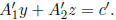
This equation can be written as the system



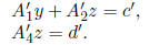
Since z is SD, we can compute z sharply from the equation using the first
method (in Section 3). We can then compute bounds on y by backsolving

When we perform the interval Gaussian elimination to obtain (8.2) from (8.1), interval
widths will tend to grow, and we should precondition. Suppose we precondition by mul-
tiplying Ax = b by an approximate inverse of the center of A. Then there is no point in
using the method just described because we can determine the hull of such a preconditioned
system sharply using the hull method. See [4].

Instead, we should precondition by an approximate inverse of the center of

where I denotes an identity matrix of order n -k. This tends to enlarge the solution set by
less than preconditioning by an approximate inverse of the center of the entire matrix A.

9. Sixth method

We now consider a method which can be regarded as a kind of dual of the fifth method.

Suppose we compute crude bounds on the inverse P of A as described in Sections 1 and
4. To simplify discussion we fix our attention on the first row of P. We also simplify by
assuming that is SD for j = 1, ..., k and that for j = k + 1,..., n:
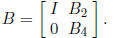
Partition A as



where is k by k and is n-k by n-k: We can perform Gaussian elimination on A in
such a way that becomes zero. This is achieved by multiplying by a matrix of the form



This matrix need not be explicitly generated. However, the operations to obtain BA must
also be performed on b so that the new equation is BAx = Bb.

The first row of the inverse PB^-1 of BA is such that its first k components are the
same as those of P and, by assumption, are SD. The last n - k components of the first
row of PB^-1 are zero (and hence SD). Since the first row of the inverse of BA is SD, we
can determine the first component of the solution of BAx = Bb by the second method (in
Section 4).

Other components of x can be bounded in a similar way.