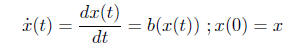
Suppose we have an ODE in R of the form
(1)
Then the solution x (t) can be thought of as function F(t,
x) of t and x that provides the
value x(t) of the solution as a function of t and x. Is F a smooth function of t
and x? It
is clear that is differentiable in t and
(2)

How about differentiability in x? If we differentiate
formally and call G = F*x
(3)
 .
.
Since F(0, x) = x, we have G(0, x) = 1 or
(4)

How do you actually prove that F*x exists and is given by the formula (4) above
? One
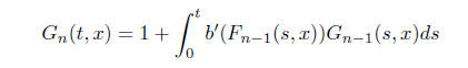
possibility is to do the Picard iteration
(5)
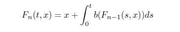
and we know that F*n → F. if we can show that
 we would be done. Denoting
 by G*n we can differentiate the iteration
formula (5) with respect to x and get
by G*n we can differentiate the iteration
formula (5) with respect to x and get
(6)
We can view (5) and (6) as just the iterartion scheme for
(2) and (3). Therefore Gn ! G.
Suppose u(t, x) is a smooth function of t and x and we consider v(t) = u(t, F(t,
x))

In particular if  In
other words any solution of
In
other words any solution of
the first order partial differential equation
(7)
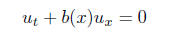
must be constant on the ”characteristics” i.e. curves (t,
x(t)) that satisfy 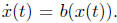
Conversely any function that is constant along characteristics must satisfy the
equation
(7).
If we have a solution (7) and we know the values of u(t,
x) at some t = T as a function
g(x), then we can determine the value of u(s, x) for any s < T by solving the
ODE (2).
At time s start from the point x and the solution of the ODE will end up at time
T at
the point F(T − s, x). Clearly u(s, x) = g(F(T − s, x)). Actually in the case of
first order
linear equations we can just as easily solve the ODE backwards in time. In fact
this just
changes b to −b. Therefore the solutions of (7) are determined if we know the
value of u
at any one time as a function of x.
All of this makes sense if x 2 R^d. Then b(x) : R^d → R^d
and the equation (7) takes the
form

Examples:
1. If we wish to solve ut + ux = 0, the solution clearly is any function of the
form
u(t, x) = v(x − t) and if we know u(T, x) = v(x − T) = g(x) then v(x) = g(x + T)
and
u(t, x) = g(x + T − t).
2*. Solve ut + (cosh x)−1ux = 0 ; u(0, x) = sinh x for t < 0 and t > 0.
It is interesting to consider a more general form of the equation
(8) < b(x),ru >= 0
in Rd and look for a solution u(x) : G ! R where G Rd and some boundary
conditions
are specified on B @G., i.e u(x) = g(x) for x 2 B. To handle this one considers
the
ODE
(9) x˙ (t) = b(x(t)) ; x(0) = x
in Rd. Clearly any solution u of (8) will be constant on the characteristics
given by (9).
If every charcteristic meets B exactly once before exiting from G and the
characteristic
from x meets B at ˆx, then clearly u(x) = g(ˆx) is the unique solution. There is
trouble
when some characteristics do not hit B, or they hit B in both directions. The
first trouble
leads to uniquness difficulties and the second to problems in existence. There
is also the
problem of what is to be done if a characteristic touches B tangentially and
comes back
inside G. Not a very clean exit!. In the earlier version with a special time
coordinate
(x0)the equation takes the form
u0+ < b(x),ru >= 0
dx0
dt = 1 or x0(t) = x0(0) + t and if the boundary is of the form x0 = c it is hit
exactly
once by every characteristic.
2
Although the ODE defining the characteristics and the first order PDE are two
sides of
the same problem they are dual in some sense. Existence for either one implies
uniqueness
for the other. This is easy to see. Because if x(t) is any charcteristic from x
( assume
for example that we are in the situation where b is continuous and we can prove
existence
without uniqueness for the ODE ) that exits at ˆx and u is any solution, then
u(x) = g(ˆx).
If u exists for enough g0s then ˆx is unique and if ˆx exists then u(x) is
determined.
It is not hard to construct trivial examples of nonuniqueness. Suppose we want
to
solve in some domain G the equation (8). Suppose b 0, then any u satisfies the
equation.
The characteristic are all constants that go nowhere. The equation reads 0 = 0
and any u
is a solution. Higly nonunique. One can construct a better example. Let us try
to solve
ut + x2ux = 0
for t < 0 with u(0, x) = 0. If we start the trajectory at some t < 0 it may blow
up before
time 0. Solving x˙ = x2 yields x(s) = (c − s)−1. x = x(t) yields c = t + x−1 and
the
trajectory x(s) = x
1+x(t−s) . Blows up when x > 0 and s = t+ 1
x . If t+ 1
x < 0 or 1+tx < 0.
it is now possible to construct a nonzero solution u. u(t, x) = 0 if 1 + tx 0.
Otherwise
we take
u(t, x) = f
x
1 + xt
if (1+xt) < 0. If we take f to be a nice smooth compactly supported function on
[−2,−1]
we have an example of a nontrivial u.
There are equations that are slight modifications that can be traeted as well.
For instance
consider for t < T and x 2 Rd,
(10) ut+ < b(x),ru > +c(x)u + d(x) = 0 ; u(T, x) = g(x)
We use a trick. Let us add two new independent variables y and z that are one
dimensional
so that we now have a problem in Rd+2. We look for a function U(t, x, y, z)
satisfying
(11) Ut+ < b(x),rxU > +c(x)Uy + d(x) ey Uz = 0 ;U(T, x, y, z) = g(x)ey + z
If u satisfies (10) then U(t, x, y, z) = u(t, x)ey + z satisfies (11). The
converse is true as
well. If U solves (11) so does U(t, x, y.z + a) − a for every a. But the
boundary values
are the same. By uniqueness it follows that U(t, x, y, z + a) = U(t, x, y, z) +
a. Therefore
U(t, x, y, z) = z + V (t, x, y). The function V will satisfy the equation
Vt+ < b(x),rxV > +c(x)Vy + d(x)ey = 0 ; V (T, x, y) = g(x)ey
If we let W(t, x, y) = e−bV (t, x, y + b), then W satisfies the same equation as
V and
therefore W = V or V (t, x, y) = u(t, x)ey for some u and then u will satisfy
(10). So let
us solve (11). We need to solve the ODE
x˙ (t) = b(x(t)) ; y˙(t) = c(x(t)) ; z˙(t) = d(x(t))ey(t))
3
If we first solve for x(·), then
y(t) = y(s) +
Z t
s
c(x(s))ds
and
z(t) = z(s) +
Z t
s
d(x( ))ey( )d
We can write
U(t, x, y, z) = g(x(T))ey(T) + z(T)
= g(x(T))ey+
R T
t
c(x(s))ds + z +
Z T
t
d(x(s))ey+
R T
s
c(x( ))d ds
Therefore
u(t, x) = V (t, x, 0, 0) = g(x(T))e
R T
t
c(x(s))ds +
Z T
t
d(x(s))e
R T
s
c(x( ))d ds
is the solution of (10).
Let us look at the simplest equation ut + aux = 0 for some constant a with the
boundary
condition u(T, x) = f(x). Then u(t, x) = f(x+a(T −t)) is the solution. We might
attempt
to solve it on a grid of points {jh, kh)} with a small h and j and k running
over integers.
For simplicity let us take T = 0. Then our equation can perhaps be approximated
by
u((jh, kh) − u((j − 1)h, kh) + a[u(jh, (k + 1)h) − u(jh, kh)] = 0
In particular
u((j − 1)h, kh) = (1 − a)u(jh, kh) + au(jh, (k + 1)h)
which allows us to evaluate u on t = (k −1)h knowing its values on t = kh. We
start with
k = 0 and work backward in time steps of h . After roughly t
h steps we should get roughly
u(t, ·) if h is small enough. Do we?
If 0 a 1, there is no problem. It is easy to show that
u(−nh, 0) =
Xn
r=0
n
r
(1 − a)n−rarf(rh) ! f(at)
( Law of Large numbers for the Binomial !)
On the other hand if a = 2 it is a mess. For example the term with r = n is
(−1)n2nf(nh)
which is a huge term. The answer, even if it is correct, comes about by a
delicate cancellation
of lots of very big terms. Very unstable both mathematically if f is not smooth
4
and computationally if we have to round off. Our discretization is stable if 0 a
1
and perhaps not so stable otherwise. In all of these cases u(jh, x) is a
weighted average
of (u(j + 1)h, ·). In the stable case the weights are nonnegative. If the
weights are both
positive and negative then the sum of the absoulte values of the weights will
exceed one
and iteration may increase it geometrically. We can buy ourselves some breathing
space
by not insisting that the lattice spacing be equal in t and x. Our grid could be
(jh, k ).
The relative sizes of and h to be chosen with some care.
Example:
3*. For solving the equation ut+b(x)ux = 0 starting from T = 0 with a value u(T,
x) = f(x)
we can construct a difference scheme of the form
1
h
[u((jh, k ) − u((j − 1)h, k )] + b(x)
1
[u(jh, (k + 1) ) − u(jh, k )] = 0.
When is this stable? For a given b how will you choose h and so that the
approximation
is stable?
5