INTRODUCTION TO MATLAB

Chapter 9
Loops and Logic

To use Matlab to solve many physics problems you have to know how to write loops and
how to use logic.

9.1 Loops
A loop is a way of repeatedly executing a section of code. It is so important to know how
to write them that several common examples of how they are used will be given here. The
two kinds of loops we will use are the for loop and the while loop. We will look at for
loops first, then study while loops a bit later in the logic section .

The for loop looks like this:
for n=1:N . . . end

which tells Matlab to start n at 1, then increment it by 1 over and over until it counts up
to N, executing the code between for and end for each new value of n . Here are a few
examples of how the for loop can be used.

Summing a series with a for loop
Let's do the sum

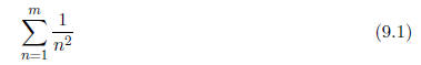
with N chosen to be a large number

You may notice that summing with a loop takes a lot longer than the matrix operator
way of doing it:

% calculate the sum of the squares of the reciprocals of the
% integers from 1 to 10,000

n=1:10000,
sum(1./n.^2)

Try both the loop way in Example 9.1a and this sum command way and see which is faster.
To slow things down enough that you can see the difference change 10,000 to 100,000.
(When we tested this, the : way was 21 times faster than the loop, so use array operators
whenever you can.) To do timing checks use the tic and toc commands. Look them up
in online help.

To get some more practice with loops, let's do the running sum

for values of m from 1 to a large number N.

Notice that in this example we pre -allocate the arrays a and S with the zeros command
before each loop. If you don't do this, Matlab has to go grab an extra little chunk of memory
to expand the arrays each time the loop iterates and this makes the loops run very slowly
as N gets big.

We also could have done this cumulative sum using colon operators and the cumsum
command, like this:
n=1:100,
S=cumsum(1./n.^2),

(but we are practicing loops here).

Products with a for loop
Let's calculate N! = 1 · 2 · 3 …(N - 1) · N using a for loop that starts at n = 1 and ends
at n = N, doing the proper multiply at each step of the way .

Now use Matlab's factorial command to check that you found the right answer:
factorial(20)

You should be aware that the factorial command is a bit limited in that it won't act on
an array of numbers in the way that cos, sin, exp etc. do. A better factorial command to
use is the gamma function -(x) which extends the factorial function to all complex values .
It is related to the factorial function by -(N + 1) = N!, and is called in Matlab using the
command gamma(x), so you could also check the answer to your factorial loop this way:
gamma(21)

Recursion relations with for loops
Suppose that we were solving a differential equation by substituting into it a power series
of the form

and that we had discovered that the coefficients a _n satisfied the recursion relation

To use these coefficients we need to load them into an array a so that a(1) = a₁, a(2) =
a₂, . Here's how we could do this using a for loop to load a(1)…a(20):

Note that the recursion relation was translated into Matlab code just as it appeared in the
formula: a(n+1)=(2*n-1)/(2*n+1)*a(n). The counting in the loop was then adjusted to
t by starting at n = 1, which loaded a(1+1) = a(2), then a(3), etc., then ended at n = 19,
which loads a(19 + 1) = a(20). Always make the code you write t the mathematics as
closely as possible, then adjust the other coding to t. This will make your code easier to
read and you will make fewer mistakes.

9.2 Logic
Often we only want to do something when some condition is satisfied, so we need logic
commands. The simplest logic command is the if command, which works like this. (Several
examples are given, try them all.)

You can build any logical condition you want if you just know the basic logic elements.
Here they are
Equal ==
Less than <
Greater than >
Less than or equal <=
Greater than or equal >=
Not equal ~=
And &
Or |
Not ~

There is also a useful logic command that controls loops: while. Suppose you don't
know how many times you are going to have to loop to get a job done, but instead want
to quit looping when some condition is met. For instance, suppose you want to add the
reciprocals of squared integers until the term you just added is less than 1e-10. Then you
would change the loop in the example to look like this

This loop will continue to execute until term<1e-10. Note that unlike the for loop, here
you have to do your own counting, being careful about what value n starts at and when
it is incremented (n = n + 1). It is also important to make sure that the variable you are
testing (term in this case) is loaded before the loop starts with a value that allows the test
to take place and for the loop to run (term must pass the while test.)

Sometimes while is awkward to use because you would rather just loop lots of times
checking some condition and then break out of the loop when it is satisfied. The break
command is designed to do this. When break is executed in a loop the script jumps to just
after the end at the bottom of the loop. Here is our sum loop rewritten with break

9.3 Secant Method
Here is a real example that you will sometimes use to solve difficult equations of the form
f(x) = 0 in Matlab. (Matlab's fzero command, which you will learn to use shortly, does
this for you automatically, here you will see how they do it.)

The idea is to find two guesses x₁ and x₂ that are near a solution of this equation.
(You find about where these two guesses ought to be by plotting the function and seeing
about where the solution is. It's OK to choose them close to each other, like x₁ = .99
and x₂ = .98.) Once you have these two guesses find the function values that go with
them: f₁ = f(x₁) and f₂ = f(x₂) and compute the slope m = (f₂-f₁)=(x₂-x₁) of the line
connecting the points. (You can follow what is happening here by looking at Fig. 9.1.) Then
t a straight line through these two points and solve the resulting straight line equation
y - f₂ = m(x - x₂) for the value of x that makes y = 0, i.e., solve the line equation to find

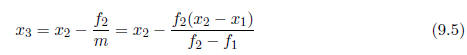
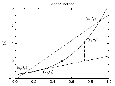
Figure 9.1 The sequence of approximate points in the secant
method.

as shown in Fig. 9.1. This will be a better approximation to the solution than either of
your two initial guesses, but it still won't be perfect, so you have to do it again using x₂
and the new value of x₃ as the two new points. This will give you x₄ in the figure. You can
draw your own line and see that the value of x₅ obtained from the line between (x₃, f₃) and
(x₄, f₄) is going to be pretty good. And then you do it again, and again, and again, until
your approximate solution is good enough.

Here's what the code looks like that solves the equation exp(-x) - x = 0

(Note: this is similar to Newton's method, also called Newton-Raphson, but when
a finite-difference approximation to the derivative is used it is usually called the secant
method.)

9.4 Using Matlab's Fzero
Matlab has its own zero- finder which probably is similar to the secant method described
above. To use it you must make a special M- le called a function, which we will discuss in
more detail in chapter 12. Here we will just give you a sample le so that you can see how
fzero works. This function le (called fz.m here) evaluates the function f(x). You just
need to build it, tell Matlab what its name is using the @-sign syntax illustrated below, and
also give Matlab an initial guess for the value of x that satisfies f(x) = 0.

In the section of code below you will find the Matlab function fz(x) and the line of code
invoking fzero that finds the root. The example illustrated here is f(x) = exp(-x)-x = 0.

Here is the function M- le fz.m used by fzero in this example: (Note: both of these
les must be stored in the same directory.)

Here is the Matlab code that uses fzero and fz to do the solve: